


Introduction
Text analysis or natural language processing (NLP) is a rapidly growing academic field that has great potential for developing novel research topics for applied social scientists and practitioners. Communication researchers have largely relied on a variety of texts—including letters, report, storytelling, textbooks, meeting logs, or even colloquial dialogue—as their primary data in their analyses. These researchers, however, have traditionally used social surveys that scrutinize communicators (rather than communication text or a “corpus” per se) or qualitative conversational analysis as their primary methods largely due to a lack of available computational or quantitative methods for text data analysis (Herring, 2004).
The situation has changed. Texts as unstructured data are now everywhere. Unlike structured data in which a limited number of data fields indicate clearly defined category or values, text data as unstructured data do not contain strictly defined data fields. Unlike structured data, many unstructured text data (such as formal letters/reports, websites or social media, informal colloquial dialogues, or online community comments) are not generated for the purpose of data analysis. It requires a specific data management process for transforming text information to numeric data, which is the topic that will be discussed in this tutorial.
This article introduces a few basic concepts and practical methods for text analysis using Python, a popular scripting language for data science (Hayes, 2020). More specifically, this tutorial provides a step-by-step guide on how to prepare the text data, how to transform strings into numeric data, and then how to summarize the frequencies of words. The data preparation procedure includes tokenization, removing stop words, stemming, and lemmatization.
Basic Steps for Text Analysis
Traditionally, limited resources did not allow social scientists to examine the entire target population and encouraged them to develop sampling methods to find out a sub-population that represents the entire target population. However, conventional sampling methods and coding schemes may not be as useful in text analysis as they are in ordinary social science survey research. Text sample data often do not represent the entire target population. For example, Annual Corporate Social Responsibility (CSR) Reports published from companies may be easily available for researchers (Vartiak, 2016) but may not represent the attitudes of all multinational companies towards CSR.
In addition, the recent development in big data storage and web scraping using R and/or Python commercial web mining tools, and database management system (DBMS) allows researchers to collect the entire census of archived text data on the web. A few examples include local newspaper articles regarding CSR in the U.S. that are available from NewsBank, official tweets mentioning CSR from the companies, archived annual CSR reports in the form of PDF files downloadable from the official websites of companies that are listed in Wharton Research Data Services (WRDS) (https://wrds-www.wharton.upenn.edu/). Web scraping techniques are beyond the scope of this tutorial. There are a number of excellent introductory textbooks in this field, and interested readers could refer to Russell and Klassen (2019).
To practice with this tutorial, readers should have Python installed on their computer. Anaconda (https://www.anaconda.com/) is a popular, open-source, and comprehensive Python package for data scientists. It is also a good choice for quantitatively oriented social scientists. Once having Anaconda downloaded and installed, we will have most of the external libraries necessary for this tutorial. We need to download and install nltk, a natural language toolkit (NLTK) library particularly for NLP (https://www.nltk.org/). Type conda install -c anaconda nltk in a command-line interface to install nltk. For interactive code writing, it is also recommended to use Jupyter Notebook, which will be installed along with Anaconda. In a code cell, type nltk.download() and finish up installing nltk.
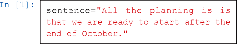
After researchers have collected text data of interest already, they will find that unstructured text data contain numerous irrelevant elements that are not useful for further analysis. To illustrate the preparation procedures for data to be analyzed, the following sentence is used as an example. It is selected from a transcribed business meeting record of a Helsinki-headquartered multinational company (Kim, Du-Babcock, & Chang, 2020).
All the planning is is that we are ready to start after the end of October.
Our sample sentence is assigned to a new string sentence in the command [1].
First, researchers may want to “tokenize” the sentence into a set of words with the command [2]. In English, words can be relatively easily tokenized by splitting the sentence by space.
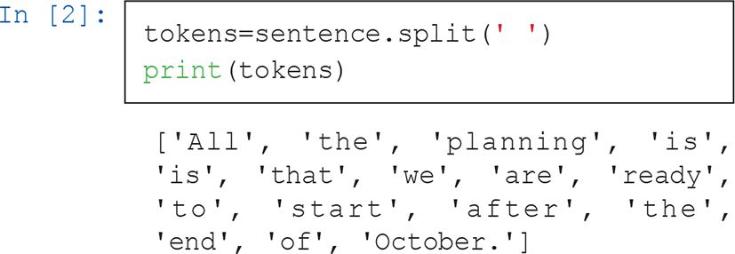
Now, a new Python list called tokens is created. The length of this list is 16, which is the number of words of the sentences. In this example, a punctuation after October ('October.') is disturbing because it makes the last element different from October in the later analysis. We can tokenize the sentence using nltk more conveniently with command [3].
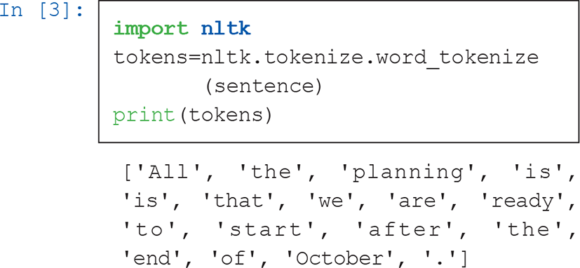
Note that this tokenization converted upper case words to the lower case. Now the length of tokens is 17 and a punctuation (.) is also counted as a word in this list independently. Note that there are two “is” reflecting the speaker’s stutter, and they are counted twice independently. Researchers may want to remove the second “is” considering the repeated be-verb is a human error, but we will handle this issue later.
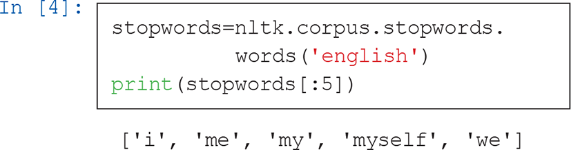
Next, we need to remove all of the stop words (a, an, the, is, are, etc.) from the sentence because they are extremely common and not substantially meaningful. There are publicly available lists of stop words online. For better performance, researchers may want to build a unique list of stop words for the purpose of their own research. For simplicity, we will use a list of stop words available from nltk in this tutorial, as shown in the command [4].
To remove stop words from tokens, we will utilize a list comprehension in Python, as shown in the command [5].
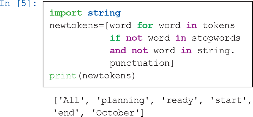
Note that we do not have stop words (the, is, that, and so forth) anymore in the result. We also used string.punctuation to remove any punctuation symbols from our example. For more delicate text manipulations, it is necessary to utilize regular expressions or re. It is beyond the scope of this tutorial, but interested readers can refer to López and Romero (2014).
Another sophisticated issue we have not considered so far is that several different wordings can be used with affixations to deliver a similar meaning in English. For example, planning is a morpheme consisting of plan and -ing. Although planning is obviously different from plan, what they refer to could be similar by context. Stemming is a useful approach for making different morphological variants consistent. There are a variety of stemming techniques; in this tutorial, we will use Porter stemmer in particular, as in command [6].
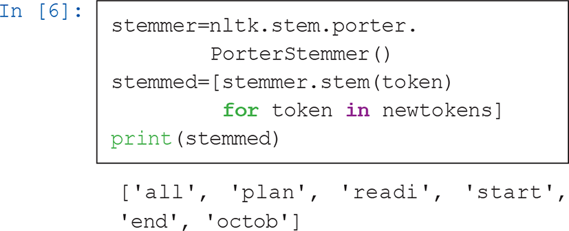
Now planning was transformed to plan (plans or planner will be transformed in the same way), ready to readi (like readiness, readily, and etc.). An unexpected error is that October is transformed to octob. This error is, however, not critical for obtaining consistency in our example because there is obviously no morphological variant in October.
One may find the stemming process too naïve because it does not take into consideration the grammatical contexts. In our example sentence, planning is a noun which connotes the presence of a formally organized policy or procedure to achieve a goal, and researchers may want to distinguish it from casual uses of plan (such as “I plan to”). We need lemmatization for this purpose. We could easily use Word Net lemmatizer from nltk with a pos, which stands for part of speech (POS) argument as shown in the command [7].
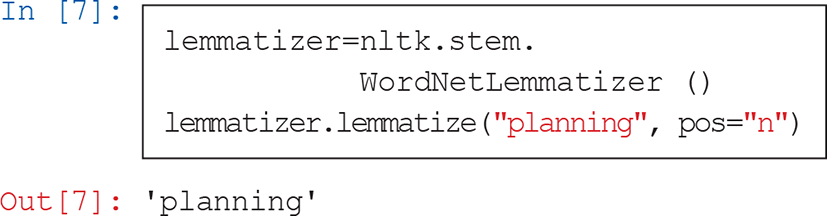
The argument pos="n" indicates that planning is used as a noun in this particular context. The result is now planning, not plan. Note that lemmatization requires accurate POS information regarding how each word is used in the context for reliable performance. However, tagging all of the words appearing in a document is often highly labor-intensive work. Although it is beyond the scope of this tutorial, there are several automated POS tagging algorithms available to end-users or researchers.
Once we prepare a list of words, we are ready to transform these string data into numeric data. The most intuitive method is what we call a bag-of-words. This approach transforms words to numbers by simply assigning a unique value to each word. For instance, we have a set of six unique words in our example:
By assigning unique values to each word, 1 is assigned to 'all', 2 is assigned to 'plan', 3 is assigned to 'readi', 4 is assigned to 'start', 5 is assigned to 'end', and 6 is assigned to 'octob'. Equivalently, a set of six words is changed to the following numeric set:
Note that the value itself is nominal and do not carry any meaningful information as it is. Therefore, researchers often prefer one-hot encoding that dichotomizes values into a series of 0 (not used) or 1 (used), as shown in the matrix below. A bag-of-words could be represented as a matrix (or so-called a document-term matrix) where each row represents a document (or an equivalent unit) and each column represents individual words used in the document. In our current matrix, there is only one row because we have one sentence in our example. It has six columns because we have six unique words in the example.
or
Now we can use a bit more of a sophisticated example to show how useful the bag-of-words approach is. The second example contains two sentences.
A: Meeting in the night before or just a full day meeting?
B: Do we start previous night? Do we start it in the night, night, the previous night?
In this example, we have two speakers and they use a variety of same and different words in the conversation. In Python, sklearn provides useful functions to extract features from texts. The sklearn.feature_extraction.text converts a collection of text documents to a matrix of token counts, as shown in the command [8].
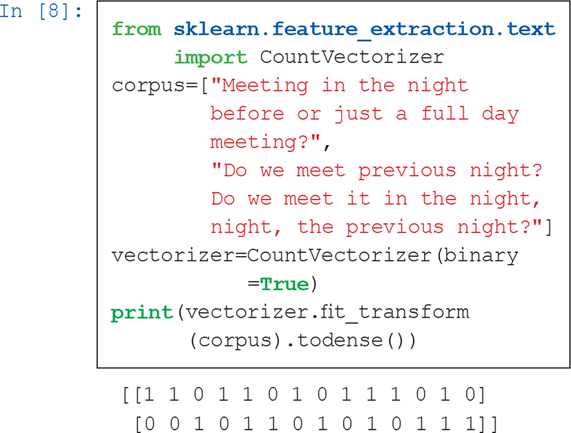
We first imported CountVectorizer from sklearn.feature_extraction.text in particular. Then we entered two sentences as two separate texts in a list (corpus). We called CountVectorizer with an argument of binary=True which dichotomizes words into the used (1) or not used (0). When we fit and transform vectorizer, we used todense() in order to obtain a dense matrix instead of a sparse matrix. The resulting matrix is as follows:
The new matrix has two rows and 14 columns because our example has two sentences consisting of 14 unique words. The result returns a series of 0 (not used) and 1 (used), but it does not show the labels corresponding each cell in the column and row of the matrix. The following command [9] prints out a list of words used and their index in the vectors.
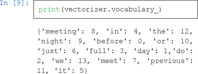
There are 0 to 13 numbers for a list of 14 elements: from 0 for before to 13 for we. Because Python counts a series from zero, the first element is 0, the second is 1, and the last element is n-1 for n elements in a list. In our example, the indices of in, night, and the are 4, 9, and 12, respectively. We can confirm that two persons use “in” (5th column of the matrix), “night” (10th column), and “the” (13th column) in common in this conversation (noted in bold).
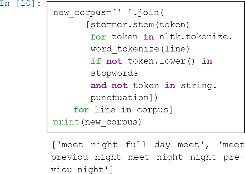
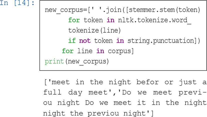
We may find this example insufficient because stop words (in, the, before) as well as substantially same words are used without stemming (meeting and meet). There are multiple methods to address this issue. In this tutorial, we will take a less Pythonic but simpler way. More specifically, we will pre-process corpus (as shown in the command [10]) before using CountVectorizer. In this command, new_corpus is generated as a list that contains multiple strings after applying stemmer.stem() and nltk.tokenize.word_tokenize().
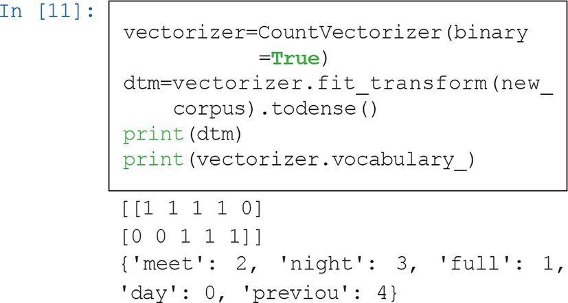
Now we can fit and transform the example sentences with CountVectorizer() as shown in the command [11]. Now this result contains no stop words, and all of the words were properly stemmed.
Note that so far we have only used single words/tokens (called unigram) when we define each cell of the matrix. We can expand to two consecutive words (bigram), three words (trigram), or more words (n-gram) to construct a bag-of-word matrix. It might be particularly useful in the context where there are some keywords consisting of more than one word—for example, “social science”, “business communication”, “data science”, and so forth. For this purpose, we can use the argument ngram_range in CountVectorizer()as shown in the command [12]. The argument ngram_range sets the length of the sequence of consecutive words in the given text. The two numbers in the parenthesis imply the minimum and maximum numbers of consecutive words.
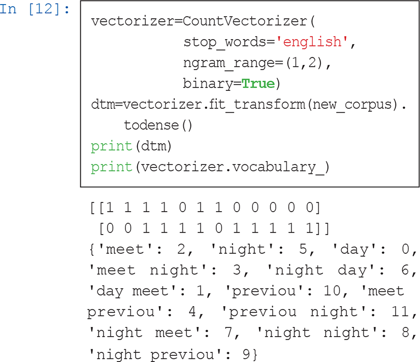
After applying n-gram of range (1, 2), the matrix of 5 columns for one words resulted from the command [11] is converted to a matrix of 12 columns including unigrams and bigrams.
So far, we have manually removed stop words that appear in the document extremely frequently but carry no substantial information. Zipf’s law states that the (log of) frequency of words is inversely proportional to (the log of) its frequency rank in various natural language contexts (Piantadosi, 2014). Frequent words are often useless to feature the unique characteristics of documents. For example, the use of “a/an,” “with,” “about,” or “for” will be not informative when classifying medical documents from military reports. However, “ambulance,” “pneumothorax,” “landmine,” or “surface-to-air” are useful for this purpose. Although they are not so frequent, words such as “prevention” would not be as useful as others because these words can often be used in both contexts.
For various purposes of text analysis, we could assume that some words are more informative when they appear frequently in specific types of documents, but not too so frequently in other types of documents. TF-IDF (Term frequency and inverse document frequency) serves this purpose (Aizawa, 2003). The formula of TF-IDF slightly differs in the literature, but the basic ideas of TF and IDF are defined as below. The TF-IDF score is defined by multiplying TF with IDF.
In this tutorial, we use sklearn to calculate TF-IDF scores. We will not remove stop words from the sentences first in this example. As shown in the command [13], we have particularly imported TfidfVectorizer class, and fitted and transformed our data with TfidfVectorizer, as we did in CountVectorizer.
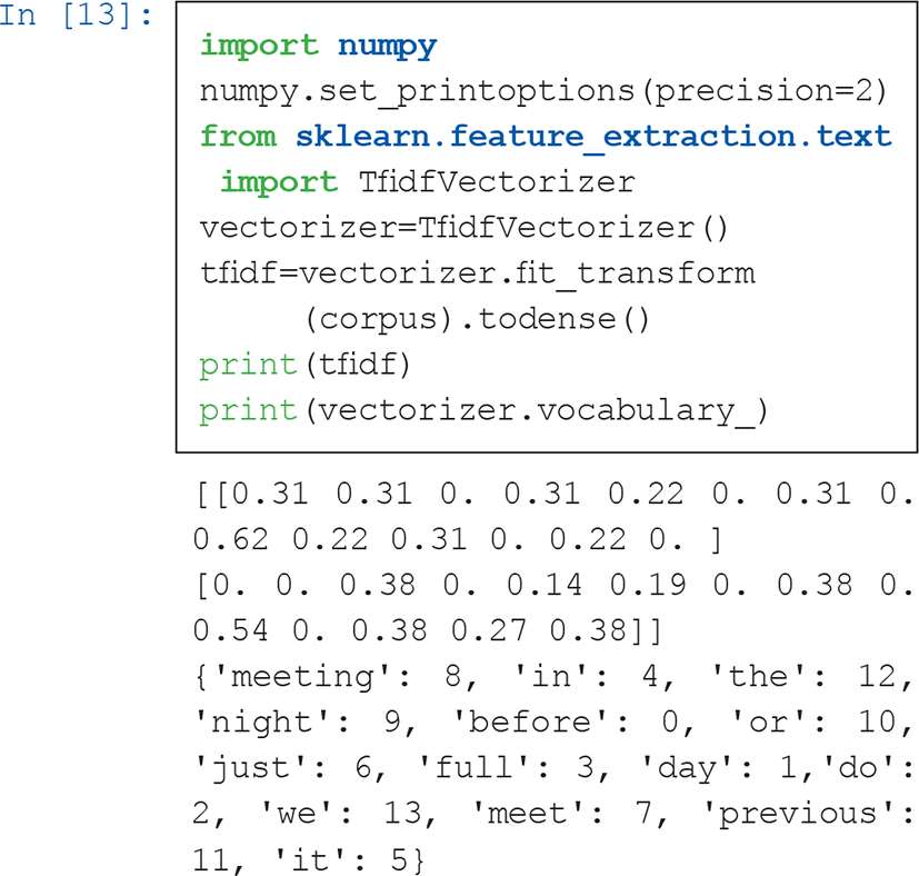
Note that vocabulary_ gives us the same result with the output from the command [9]. We can compare the document-term matrix (above matrix (4)) with this TF-IDF score matrix (5).
Some words (or tokens) have obvious higher TF-IDF scores (for example, TF-IDF score of meeting for A is .62 and that of night for B is .54) than other words. As shown in Example 2 and the corpus in the command [8], the word meeting was used twice only by A, and night was used four times by B, although A used night just once. These two words “feature” the unique characteristic of each document (or each person in our example), therefore have higher TF-IDF score. Interested readers can conduct the analysis again after stemming meeting to meet, as shown in the command [14],
Now we have a numeric data set representing the presence/absence or how important individual words/tokens are in various contexts, as shown in matrices (4) or (5). We can perform various statistical methods or machine learning algorithms to regress, cluster, or classify the data sets.
Discussion
In the era of big data where people, devices, infrastructures, and sensors constantly communicate and generate data, data analysis is now the keyword and trend of the times for those not only in the field of data science but also in all functions of the business industry who wish to find hidden insights from data. An increasing amount of research has also shown significant value in using a big data analytics approach to examine the business communication process. With texts as unstructured data everywhere, text analysis or NLP is a rapidly growing academic field that has great potential for novel research among many applied social scientists and practitioners.
Text mining is a technology aimed at extracting and processing useful information from text data based on NLP technology. Since many unstructured text data are not generated for the purpose of data analysis unlike structured data, text data needs to be converted to numeric data through the process explained in this paper. In this process, anyone who wants to start analyzing the raw data should decide whether to learn R or Python (or both of them), which are representative open source tools of data analysis at present. The choice of R or Python depends on the type of data and the nature of the task. Typically, R is a tool that contains more statistical elements, and Python has good accessibility with an easy to understand and flexible syntax for more generalized scientific computing. In this tutorial, Python was used to show the NLP process because it has the advantage of performing tasks using available packages or libraries and is an intuitive programming language that even beginners can learn easily.
As shown in this paper, the bag-of-word method or TF-IDF method is an important starting point for NLP, and they still have great potential for various quantitative or computational analyses—for example, simple word frequency analysis, word network analysis (Drieger, 2013), language detection (Stensby, Olmmen, & Granmo, 2010), speech recognition (Washani & Sharma, 2015), or naïve Bayes spam filters (Rusland, Wahid, Kasim, & Hafit, 2017). After getting used to the topics covered in this tutorial, interested researchers will find more advanced topics such as sentiment analysis (Gupta, 2018), latent Dirichlet allocation (LDA) (Blei, Ng, & Jordan, 2003), and word embedding (Karani, 2018). Analyzing the text data in the business environment, the NLP process will provide new opportunities and increase potential for business growth.
Conclusion
By following the procedure described in this paper, it is possible to analyze a variety of text data using Python. With a numeric data set representing the presence/absence or how important individual words/tokens are in various contexts, communication researchers can perform various statistical methods or machine learning algorithms to regress, cluster, or classify contents of data sets. In addition to the data preparation procedures of texts, the bag-of-word or TF-IDF methods are important starting points for NLP and they still have a great potential for various quantitative or computational analyses. As a mild introduction, this tutorial does not require any serious knowledge in the field. For advanced text analysis, however, studying introductory statistics, computational linguistics, and R and/or Python is strongly recommended.